Automatic detection of spontaneous postsynaptic currents
Introduction
The release of neurotransmitters happens primarily when action potentials invade the neuronal presynaptic terminals. Nonetheless, neurotransmitters can also be released "spontaneously", in absence of action potentials or significant depolarization of the presynaptic membrane. This "spontaneous" neurotransmitter release can be measured with intracellular (generally patch-clamp) recordings from postsynaptic neurons in form of transient postsynaptic currents (PSCs). These events can be distinguished in spontaneous PSCs (sPSCs) or, if measured in presence of Na+ channels blockers, miniatures PSCs (mPSCs).
Electrophysiologists have found out that the frequency, the amplitude and the kinetics of these transient events can provide important insights in the physiological properties of synapses. Furthermore the experimental settings required to measure them, is relatively easy. For these reasons, recording sPSCs or mPSCs is often the experiment of choice for in vitro electrophysiologists interested in studying synaptic function.

The detection of sPSCs / mPSCs is time consuming and its automation is not trivial.
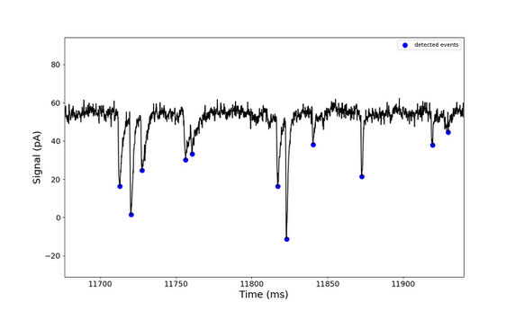
For this reason, I developed a tool, primarily based on a deep learning model, to optimize the automation of this analysis. Here, an example of automatic detection from a short current trace's segment.
Where to get the tool
If you would like to use this tool, you can find the source codes and a detailed explanation on how to use it at: https://github.com/Imbrosci/spontaneous-postsynaptic-currents-detection.
The tool is easy to use even for people with very little programming experience. Furthermore, the results are automatically saved in an excel file and possible residual errors can be corrected interactively.
How the deep learning model works
Model training

To build this tool the first step was to generate a large dataset to train a deep learning model.
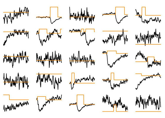
The samples used to train the model are short time series, representing 15 ms long segments of current traces, and the targets are binary vectors of the same length filled with 1s in correspondence and proximity of sPSCs / mPSCs peaks and with 0s otherwise.
The image represents few samples used to train the model (in black, the current traces's segments and in darkorange, the binary targets).
Model prediction
For model training and validation, the dataset was then splitted in training (85%) and validation (15%).
The output of the model is a probability (ranging from 0 to 1) for each data point. The higher the probability, the higher the likelyhood of a data point to be
within a sPSCs or a mPSCs.
To process a long current trace, the strategy was to feed the neural network with segments from the current trace, in a sliding window fashion, as demonstrated in
this short video below. The prediction of the neural network is the probability trace (in darkorange).

Finding single sPSCs / mPSCs
To detect single events, there are still some postprocessing steps to do. First of all, a threshold from the prediction trace is chosen (darkgreen).

After setting this threshold, an algorithm will search and filter peaks from the prediction trace following specific criteria. The found peaks will then be further evaluated by a second deep learning model (to exclude as many false positives as possible). The peaks passing this last "filter" will be the detected as sPSCs / mPSCs (dark green).

